The Transit of Mercury

May 9th 2016

by Martin J. Powell

On May 9th 2016 a transit of Mercury across the face of the Sun took place. Mercury transits are relatively rare events which can be observed from much of the world, however since they involve viewing the Sun, extreme caution must be taken when attempting to observe them (for details on how to safely view the Sun, see below).

During a transit, Mercury is seen as a tiny black dot moving slowly in an East-to-West direction across the Sun. The 2016 transit commenced on May 9th at 11:12 UT (Universal Time, which is equivalent to Greenwich Mean Time) and ended later that same day at 18:42 UT, with mid-transit taking place at 14:57 UT. The total duration was therefore about 7½ hours, however because of the effect of parallax, the exact duration varied by ±2 minutes depending upon the observer's location on Earth. The planet crossed the Sun in a North-east to South-west direction, as opposed to a South-east to North-west direction at the previous transit in November 2006. This is because May and November transits of Mercury are viewed from opposite sides of the Earth's orbit, Mercury being seen descending (moving North to South) during May transits and ascending (moving South to North) during November transits. After 2016, the next two Mercury transits will take place on November 11th 2019 and November 13th 2032.

Because Mercury is seen against the solar disk, a transit can be viewed from anywhere on the Earth where the Sun is above the horizon at the time of the event. The 2016 transit could be seen in full from Western Europe (including Scandinavia), extreme North-west Africa, Eastern North America, Northern South America, Greenland and the Arctic (the Sun being above the horizon throughout). At latitudes North of about 73° North the Sun is above horizon throughout the day at this time of year, hence the entire transit was visible. For much of the inhabited world, however, the transit was already in progress at sunrise or sunset so it was not seen in its entirity. The event could not be seen at all from Australasia, extreme Eastern Russia and China, Japan, the Korean peninsula, the Philippines, Eastern Malaysia, Indonesia and most of Antarctica because the Sun was below the horizon from these locations.

The German astronomer Johannes Kepler (1571-1630) was the first person to predict a Mercury transit event, although he did not observe one himself. His prediction of a transit on November 7th 1631 enabled the French mathematician and astronomer Pierre Gassendi (1592-1655) to observe it, in the year following Kepler's death.

Circumstances of Mercury Transits

Transits of Mercury can only occur whenever the planet is close to its ascending node or descending node (the points in its orbit where the planet crosses the ecliptic - the apparent path of the Sun against the background stars) heading Northwards or Southwards, respectively. For such an event to take place, the planet must be close to inferior conjunction (i.e. positioned directly between the Earth and the Sun) and also be positioned within about 2° of one of these nodes. Because of the positioning of the nodes in relation to the Earth's orbit, in the present era transits can only take place in the second week of May (descending node) or in the second week of November (ascending node). The ascending and descending nodes of the planets are positioned exactly 180° apart - hence the six-month difference between these two dates. Because the node positions change very slowly over time, the dates of Mercury transits are drifting later in the calendar. In the 18th century, for example, transits took place between May 2nd and 7th, whereas in the 21st century they occur between May 7th and 10th, a drift of about 1½ days per century.

At the moment of mid-transit in 2016, Mercury was positioned about 0°.9 away from its descending node (measured relative to the Sun's centre), the planet having passed through the node some 3½ hours before the start of the transit. Viewed from the Earth, the node was positioned some 29 arcminutes (29' or 0°.48) ENE of the Sun's apparent centre. Mercury transits at the descending node take place when the Sun and Mercury are positioned in the constellation of Aries, the Ram whilst those at the ascending node take place when the two celestial bodies are positioned in Libra, the Balance.

November transits of Mercury repeat at intervals of 7, 13 and 46 years whilst those in May repeat at intervals of 13, 33 and 46 years. November transits outnumber May transits in the approximate ratio of 7:3. May transits are slower than November transits because Mercury is then closer to the aphelion point in its orbit (i.e. its furthest point from the Sun) and its orbital speed is therefore slower (the longest possible duration of a May transit is a little under 9 hours). Conversely, November transits are swifter because the planet is then near perihelion (its closest point to the Sun) and so its orbital speed is faster. The 2016 transit lasted about 2½ hours longer than the previous one on November 8th-9th 2006; the track (chord) of Mercury also passed closer to the Sun's centre and was therefore slightly longer.

Venus can also be involved in solar transits, since it also passes directly between the Earth and the Sun; this last occurred in June 2012 and will next occur over a century later, in December 2117. Mercury, however, appears much smaller than Venus when viewed from the Earth so optical aid is always required to view the event. Transits of Mercury are much more common than those of Venus - during the 21st century, for example, there are fourteen Mercury transits but only two Venus transits (in 2004 and 2012).

During the 2016 transit Mercury had an apparent diameter of 12" (12 arcseconds). The Sun's apparent diameter at this time of year is 31'.7 (i.e. 1900") which means that the Sun's apparent disk was approximately (1900 ÷ 12) = 158 times larger than that of Mercury (to gain a sense of just how small the planet appeared on the solar disk, see the scale diagram here). Because of parallax, Mercury's disk appeared very slightly displaced in a vertical sense on the solar disk when seen from locations in the far North and far South of the world. For example, an observer situated in Nome, Alaska, USA saw Mercury positioned 22" further South on the Sun's disk than an observer situated at Santiago, Chile - an angular distance which is equivalent to almost two apparent Mercury-diameters. All of the diagrams on this page show Mercury positioned in a geocentric sense, i.e. from a theoretical position at the Earth's centre.

Note that, although mid-transit occurred on May 9th at 14:57 UT, it did not coincide with the moment of Mercury's inferior conjunction; this took place at 15:13 UT, some 16 minutes after mid-transit. At its closest point, Mercury passed 5'.3 South of the Sun's centre.

^ Back to Top of Page

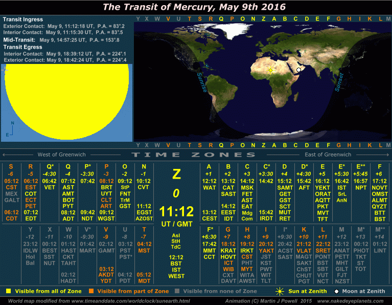
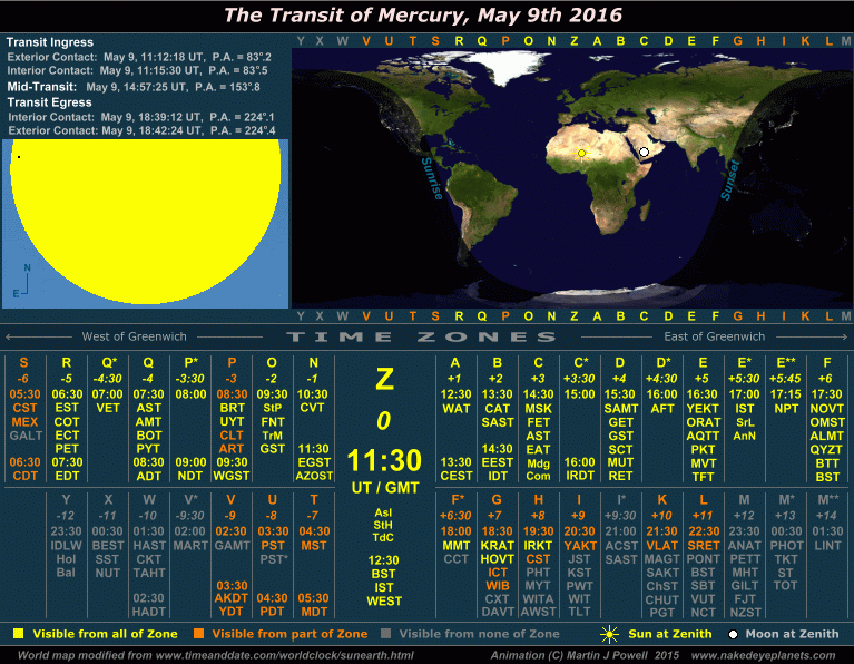
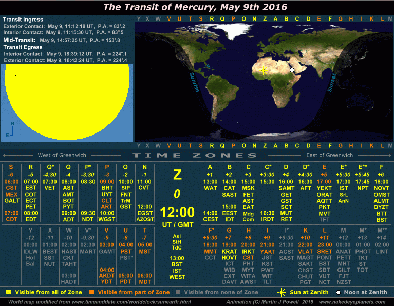
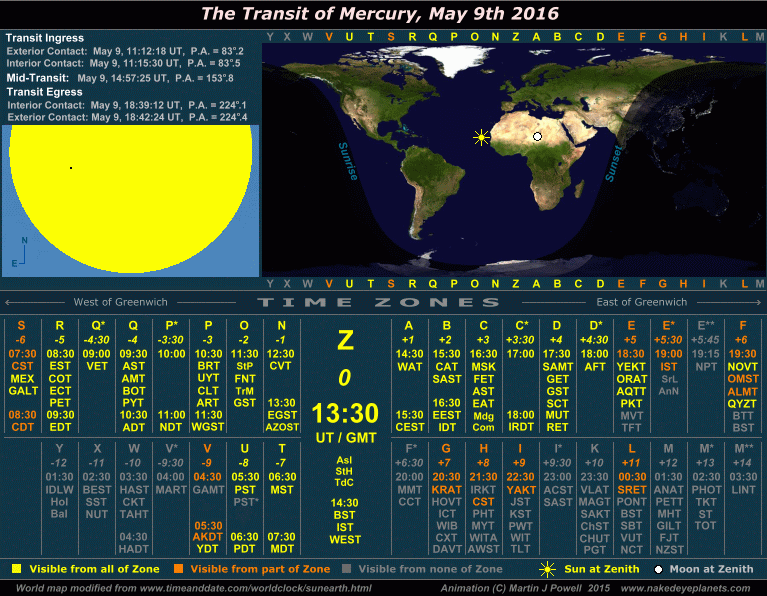
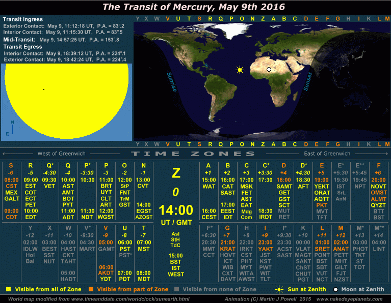
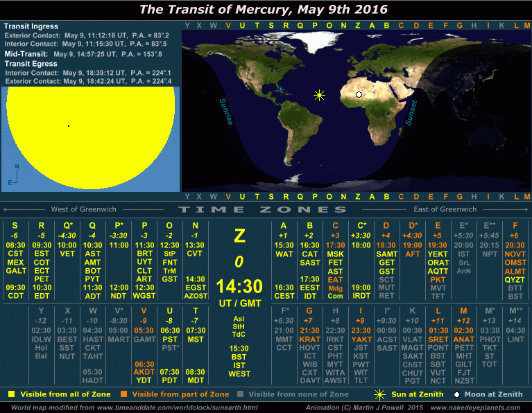
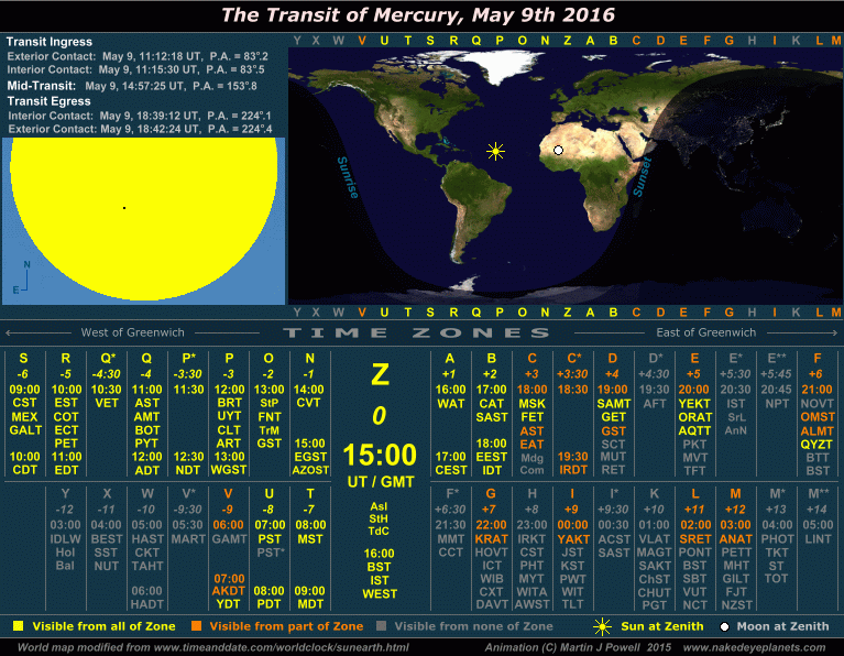
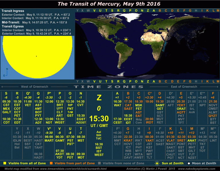
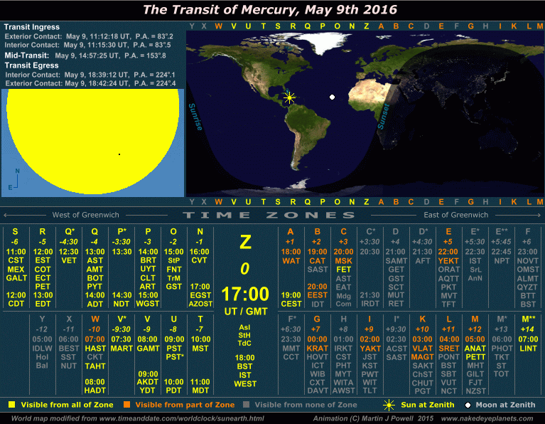
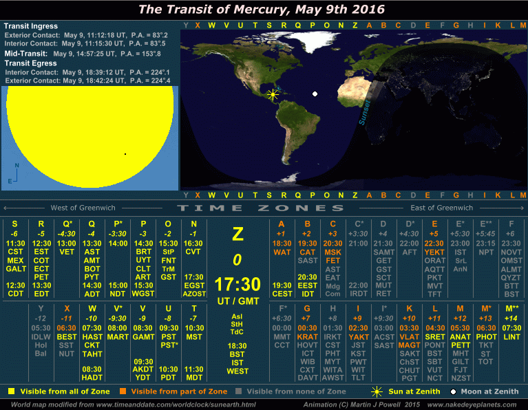
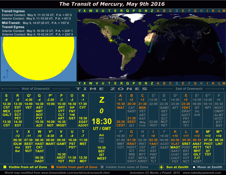
The Mercury Transit 2016 World Time/Visibility Map

The time/visibility map shows the changing events over the course of the transit. As Mercury moves across the Sun's disk, the Earth's shadow moves accordingly across the world map and the local times across the world are displayed at each stage. It commences on May 9th at 11:12 UT (at the start of the transit), after which there is an 18-minute interval (to 11:30 UT). The next 6½ hours (12:00 UT through to 18:30 UT) are shown at half-hourly intervals, after which there is a 12-minute interval, bringing the time to 18:42 UT (the end of the transit). The time/visibility map therefore allows one to estimate the times at which the transit was visible from his/her own location to within about 30 minutes.

The start of the transit (i.e. when the disk of Mercury moves on to the solar disk) is known as the ingress whilst the end (when Mercury moves off the solar disk) is known as the egress (see illustration at right). Both ingress and egress are divided into exterior contact (where Mercury's disk is externally tangential to that of the Sun) and interior contact (where Mercury's disk is internally tangential to that of the Sun). Timings of the ingress, mid-transit and egress are given in the box at the upper left of the time/visibility map (times are shown in UT). Also shown is the position angle (P.A.) of Mercury on the solar disk, i.e. its compass bearing relative to the Sun's centre (measured anti-clockwise from North through East, South and West, where North = 0°, East = 90°, South = 180° etc). Beneath the ingress and egress times the lower section of the Sun's disk is shown, with Mercury appearing as a tiny black dot (shown to scale). The world map beside it shows which regions were in daylight or night-time as the transit took place.

Beneath the illustrations, the time zones of the world are shown. Each time zone extends 15° in longitude (i.e. equivalent to one hour of the Earth's rotation). In the time/visibility map, the zones are listed according to their military designations (where A = 'Alpha', B = 'Bravo', C = 'Charlie' etc). Under this scheme, time zone Z ('Zulu') represents Greenwich Mean Time; this zone is centred on the Greenwich Meridian (0° longitude). Time zones A to M are situated to the East of Greenwich (i.e. to the right of 'Zulu' time in the time/visibility map) whilst zones N to Y are to the West of Greenwich (i.e. to the left of 'Zulu' time in the time/visibility map). Because of space limitations, the time zones in both East and West regions are split into two, one above the other. For quicker identification, the approximate locations of each time zone is marked above and below the world map.

Each time zone column is headed by its military letter designation. Beneath it, in italics, is the standard time difference from Greenwich (i.e. not the summertime offset). Hence at New York, USA, the standard time difference from Greenwich is -5 hours (5 hours behind Greenwich) and it therefore falls under time zone R ('Romeo'). Beneath the italicised time offset is displayed the Standard Time operating in that zone; hence in the above example (zone R) it will be 5 hours behind the Greenwich time. Since it was summertime in the Northern hemisphere, Daylight Savings Time operated from numerous locations in the Northern hemisphere and wherever this applies it is shown at the bottom of the column. Hence in zone R, Eastern Daylight Time (EDT) was operating, which is one hour ahead of the Standard Time.

Within each military time zone column, up to six local time zones are shown. These are typically the six most populous local time zones within that military zone, listed in order of approximate latitude from North to South (local time zones with little or no internet presence have been excluded). Hence in military time zone D ('Delta') the local zones SAMT (Samara Time), GET (Georgia Time), GST (Gulf Time), SCT (Seychelles Time), MUT (Mauritius Time) and RET (Réunion Time) are listed, these being the most populous local zones within that military time zone - SAMT (Western Russia) being furthest North in latitude and RET (Réunion Island) being furthest South. In some instances only one country operates a particular time zone; hence in time zone E** ('Echo star star') Nepal is the only country operating its time offset of +5:45 hours, so only the abbreviation NPT (Nepal Time) is listed. Where space allows, individual islands are listed, even where they operate on the same local time zone as their parent country.

The time zone lettering is colour-coded to indicate whether the transit was wholly visible, partly visible or not visible from any given military and/or local time zone (the military time zone letters above and below the world map also change colour accordingly). Because the Earth's shadow fell obliquely across the time zones at this time of the year, in many cases one region of a time zone could see the transit whilst another region could not, despite the clock times being the same; wherever this situation occurred, the time zone data appears orange. For example, from India (military time zone E*, local zone IST) the start of the transit (at 16:42 IST) was visible so the initial period is shown in yellow. The start was also seen from Sri Lanka (SrL) and the Andaman & Nicobar Islands (AnN) - both of which use the IST time zone - so they are also shown in yellow at this stage. The transit was visible from all three locations until 18:00 IST, by which time the Andaman Islands had lost sight of the Sun (at sunset), hence the 'AnN' designator turns grey. By 18:30 IST the Sun had also set over Sri Lanka and Eastern India, so the 'SrL' designator turns grey whilst the IST designator turns orange (i.e. it was only partly visible from mainland India). The IST designator remains orange for an hour until 19:30 IST, by which time the Sun had finally set across the remainder of the country. Henceforth the IST designator - along with all the other data in the column - is shown in grey.

The transit was wholly visible from time zones Z (with the exception of a couple of remote islands), N ('November'), P* ('Papa star'), Q ('Quebec') and Q* ('Quebec star'); consequently, these zones appear yellow throughout the time/visibility map. The transit was not visible from time zone I* ('India star', i.e. local zones ACST and SAST in central Australia) since it took place during the local night time, hence it is coloured grey throughout the time/visibility map. From all other time zones, the transit visibility changes between not visible, partly visible and/or wholly visible, depending upon where the region was situated in relation to the Earth's shadow at any particular time.

The line (curve) dividing the light and dark regions of the world (or of any planet or moon, for that matter) is known as the terminator. On the world map it is labelled Sunrise on the shadow's Eastern edge and Sunset on the shadow's Western edge. It follows that the closer to the terminator a particular daylight region of the world is positioned, the lower in the sky the Sun would have appeared from that region.

Close to the Northern edge of the shadow, where daylight is almost continuous at this time of year, the Sun set during the transit and then rose a couple of hours later with the event still in progress, e.g. in the Sakha Republic of North-eastern Russia (local zone VLAT, military zone K). Conversely, along the Southern edge of the shadow, the daylight is short at this time of the year. Along the ice-cliffs of the Princess Märtha Coast in Antarctica, the Sun rose during the transit and set a few hours later, so that the event was visible for the entire local daytime.

Note that from several time zones the transit was not seen entirely on May 9th. Across Northern Russia in time zones G ('Golf'), I ('India'), K ('Kilo') and L ('Lima') the transit was first seen on May 9th local time and was last seen on May 10th local time. From time zones M ('Mike'), M* ('Mike star') and M** ('Mike star star') which straddle the International Date Line, only the latter part of the transit was seen after sunrise on May 10th local time.

Finally, the zenith position of the Sun (i.e. where it was positioned directly overhead) is shown on the world map by the symbol . On May 9th 2016 at 15:00 UT the Sun's declination (angle from the celestial equator) was +17°.5, which means that the Sun passed through the zenith around midday from all locations along latitude 17°.5 North (it was overhead at Niger at the start of the transit and overhead at Mexico at the end of the transit). The zenith position of the Moon is likewise shown by the symbol .

More precise transit times for various cities across the world can be found at the following websites:

• The EclipseWise website lists the Mercury transit times and Sun altitudes for over 80 USA cities and over 100 Canadian cities, all in local times.
• The US Naval Observatory (PDF file) lists the local circumstances for 32 USA cities and numerous cities worldwide, with times in Universal Time (UT).

^ Back to Top of Page

The 'Black Drop Effect'

During a solar transit, both Mercury and Venus are subject to a mysterious phenomena known as the black drop effect. First observed during a transit of Venus in 1761, it occurs just after the moment of second contact (ingress, internal contact) and also just before the moment of third contact (egress, internal contact). Seen at high magnification, Mercury sometimes appears elongated in the direction of the Sun's limb, causing the planet to appear momentarily 'teardrop-shaped'. The apparent 'ligament' between the planet's limb and the Sun's limb appears greyish and fuzzy, often frustrating astronomers' attempts to determine the precise moment of second and third contact. In the case of Venus, the scientific theory for many years was that the phenomena was caused by sunlight refracting through Venus' atmosphere in the direction of the Earth, thus distorting the planet's apparent shape. However, the high number of observations by amateurs and professionals during the planet's 2004 transit began to cast some doubt on this explanation. Whilst smaller telescopes users were often seeing the 'black drop', many observers using larger instruments did not.

The mystery was largely solved when astronomers studied the results of an Earth-orbiting satellite observation of a Mercury transit in 1999. Unlike Venus, Mercury does not have any significant atmosphere but the effect was nonetheless observed - hence the 'black drop' could not have been caused by atmospheric refraction. Neither did the Earth's atmosphere play any significant role (i.e. turbulence or poor seeing conditions) since the satellite observing Mercury was, of course, orbiting the Earth! The astronomers concluded that the 'black drop' was caused by a combination of two factors: a telescope's inherent optical defects (causing any image seen through it to be slightly blurry) and solar limb darkening, i.e. the darkening effect around the Sun's circumference (limb) caused by the gas in that region being more opaque - and therefore darker. These two factors combine to cause a dark blurriness at the point where the limbs of Mercury and the Sun touch - hence causing the 'black drop effect'.

^ Back to Top of Page

Observing the Mercury Transit

The safest way to observe a transit of Mercury (or Venus) is to project the image of the Sun through a refracting telescope on to a piece of white card (i.e. the image of the Sun is projected backward through the telescope, from the main object glass through to the eyepiece and on to the card). In practice, a second piece of card is normally attached to the telescope, positioned just ahead of the eyepiece and perpendicular to the telescope's axis, in order to create a shadow around the projected image and thereby improving its contrast. The solar image on the card appears pale white, the silhouette of Mercury looking like a small black dot (rather like a sunspot). The projected image may be flipped horizontally and/or vertically, depending upon the telescope's optical arrangement.

Binoculars can similarly be used to project the Sun on to a piece of card. The resulting image is naturally smaller than that from a telescope and, of course - unless one of the lenses is capped - the binoculars produce two identical images.

Transits can also be observed safely through a telescope by attaching an aluminised mylar solar filter to the front of the telescope, ahead of the object glass (always ensuring beforehand that the filter has not been damaged in any way!!). If an aluminised solar filter is used the solar disk may appear pale blue, pale yellow or white, depending upon the manufacturer's specific design. Filters can also be purchased which can be attached to conventional cameras for photographing the event.

The apparent size of Mercury's disk during a transit - only one-fifth of that of Venus at its 2012 transit - is too small to be seen with the naked eye. Consequently, commercially-available filters allowing direct viewing of the Sun using a pair of cardboard 'spectacles' (solar viewers or eclipse shades) is of no use in observing a transit.

The UK's Open University produced a short video describing how to safely view the 2016 transit. More information on how to safely view the Sun can be found at NASA's website.

Internet Live Broadcasts

The following websites broadcast the 2016 transit live on the Internet:

^ Back to Top of Page

Sources

• Useful information on past, present and future Transits of Mercury were obtained from 'The Handbook of the British Astronomical Association 2016', pgs. 12-3, the article 'The transit of Mercury on 2016 May 9' by Peter Macdonald in 'Journal of the British Astronomical Association', Vol. 125, No. 5 (October 2015), pg. 263, 'Norton's 2000.0' edited by Ian Ridpath (Longman Group UK Ltd., Harlow, 1989), pg. 101, 'The Guinness Book of Astronomy Facts and Feats' by Patrick Moore (Guinness Superlatives Ltd., Enfield, 1983), pg. 54 and 'Astronomy and the Imagination' by Norman Davidson (Routledge & Kegan Paul, London & New York, 1985), pg. 202. Other useful sources included the SkyGazer Ephemeris utility by John Biondo and the website The Sky and Its Phenomena by Italian amateur astronomer Pierpaolo Ricci (where a list of Mercury transit dates/times can be found for the years 1907-2295 AD).

• The diagram showing the planets in their orbits at the time of the transit was based on Dirk Matussek's AstroViewer^® Java applet (Solar System tab).

• The transit tracks illustrations and parallax measurements were derived from the commercial software RedShift 5 by Maris Technologies Ltd.

• The regions of the world from which the 2016 transit can be seen were assessed using the time zone map from the United States Naval Observatory website using additional time zone information from WorldTimeZone.com and TimeandDate.com.

• The world map images used in the time/visibility map were modified from the 'day and night world map' at TimeandDate.com.

Copyright  Martin J Powell  December 2015